ExcelFrog Clear Excel Tutorials

home about

Excel: How to Format Your Data in 60 Seconds

Having important data in Microsoft Excel is cool, having it look nice and clean without spending 2 hours on formatting is even better. In this short tutorial we will see how to make your data look great, step-by-step, in less than 60 seconds of work. It's also a good way to understand the basics of Excel formatting.

Here's our subject, a boring Excel table:

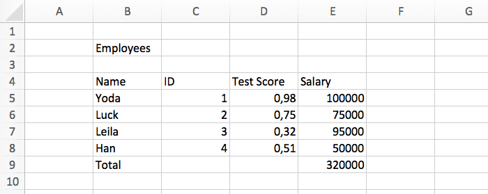
Let's see how it will look like by the end of this tutorial :-)

The Header

The header of the table needs to stand out. To do so, first center the text and make it bold.

Then, to make it even more visible, we can change its colors. A dark background with a white text works great for this. However try to avoid flashy colors in your spreadsheets, they tend to be distracting.

The Data

The actual data in the table is the most important information, that's why it has to be really easy to read. The best way to achieve that is to format it correctly. So set the percentages as percentages, and the amounts in dollars.

Don't forget to round the numbers to avoid cluttering the cells.

The Footer

The last row of the table contains the total, and it should not be confused with the other rows. So we need to style it a little differently. First make the text italic.

Then add a top border to further separate it from the data above.

Finishing Touches

We are almost done, just a couple more things to do.

Make the title of the table look nice with Excel built in styles. Feel free to explore the other styles available, they can be quite useful to quickly format a cell.

And add a thick border to the whole table to make it stand out. It's a small change that makes a big difference.

Bonus

In case you made a mistake and want to quickly change the style of a cell, you can easily do so with the very useful brush tool. Here's how it works: select a cell with the correct style, click on the brush tool, and select the cells you want to change.

Conclusion

You can see below the comparison between the original table and the new one.

The end result looks much better, and it is also clearer. You can do the exact same thing to your own data in less than 60 seconds. I actually just timed myself, and it took me 42 seconds from start to finish ;-)

FYI here's a quick summary of what we did:

• Header: bold text, center text, dark background color, white text.
• Data: number formatting, number rounding.
• Footer: border top, italic text.
• Other: title cell, thick table border.

See all the tutorials on the homepage