 ExcelFrog
Clear Excel Tutorials
ExcelFrog
Clear Excel Tutorials
When using Microsoft Excel, you often have to deal with huge tables full of data, and things can get pretty hard to manage. In this short tutorial we'll see 3 Excel features that can help you better handle large spreadsheets.
Here's the big table that we are going to work with:
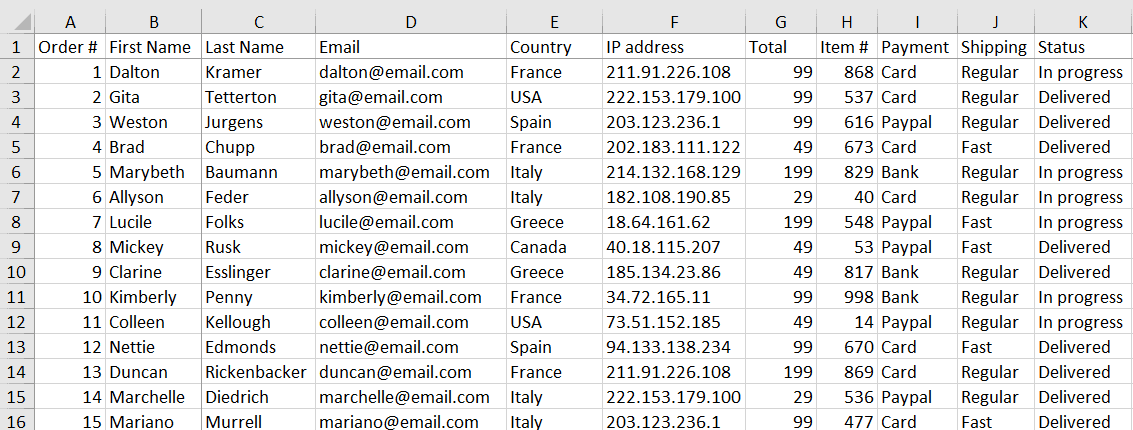
Take a deep breath, and let's go!
Once you start to scroll vertically or horizontally in your dataset, it's really easy to get lost. One simple solution is to freeze the most important rows and columns so that they are always visible on the screen.
First we have to decide which rows/columns we want to freeze. In our example we might want to see the top row and the first 2 columns. To do so, you have to select the first cell that should not be freezed (in this case it's the cell C2), then click on the "freeze panes" button in the "view" tab.
And now when we move around, the most important information is always visible.
The table we are working with has 11 columns. Do we really need all of them? Probably not. But we don't want to delete them either, they can become useful later. That's why there's a cool feature in Excel to temporary hide columns.
Simply select all the columns you want to remove by clicking on them while pressing ctrl (or ⌘ on a Mac). Then right click to select "hide".
To undo this, select the columns right before and after the ones that are hidden, then right click to select "unhide".
The last thing we should do is to filter all this information, so we can focus on the rows we actually need.
Make sure the active cell is somewhere in the table, and go in the "data" tab to click the "filter" button. You'll see all the cells in the top row get a small arrow next to them.
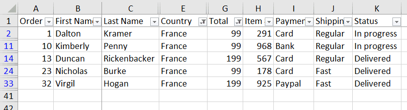
When you click on the small arrow, you can select exactly what you want to see. In the example below I'm interested only in customers from France who ordered more than $75 of goods.
In this tutorial we managed to transform a huge spreadsheet into a small table containing exactly the information we needed. So this is going to be much easier to parse and analyze. Pretty cool, huh?
Here's a quick summary of what we covered: