 ExcelFrog
Clear Excel Tutorials
ExcelFrog
Clear Excel Tutorials
In our previous tutorial, you've seen 5 settings in Microsoft Excel that may help you get a better spreadsheet experience.
In this second part of the tutorial, you will find 5 more advanced settings that may be your timesaver and even protect your Excel files from crashing!
In Excel, a circular reference occurs when you enter a formula in a cell that links directly or indirectly to itself. This creates an endless loop of calculations between multiple cells.
Usually we create circular references by mistake, but their impact can be destructive. The processing speed of Excel will largely slow down and the endless iterative calculations may directly crash your workbook. Pretty scary, huh? Here's a tip to help you!
Click File > Options > Formulas. In the "Calculation options" section, make sure the "Enable iterative calculation" option is unchecked.
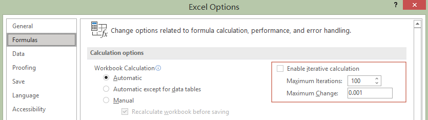
This will prevent Excel from doing iterative calculations every time a circular reference is created, and you will be informed with an error message at the same time.
I recommend to keep this box unchecked at all time. Note that once you turn it on you will not get any more warnings about circular references.
Of course, this setting will just help us detect circular references, but not to fix them. I will share with you some tips to kill circular references in the future!
By default, Excel allows you to edit the data of a cell when you double click on it. But when you do some formula auditing, you may prefer to check the elements of the formulas rather than edit the data itself.
Here's an example, when you double click on the net salary amount (C4), by default the formula Net salary = Gross salary (C2) * (1 - Tax rate(C3)) will show in the cell which allows you to edit it directly.

But instead, you may want to locate the elements "Gross salary" and "Tax rate" to audit the formula. Like this:
To do so, click File > Options > Advanced. In the "Editing options" section, uncheck "Allow editing directly in cells" box.
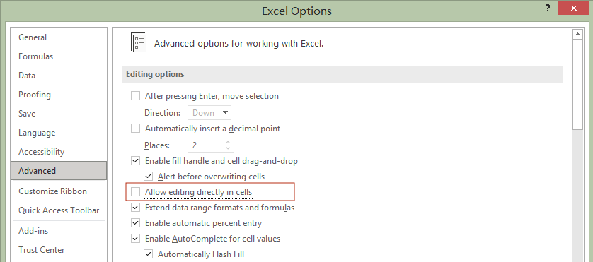
Now if you double click the cell C4, the cells of Gross salary (C2) and Tax rate (C3) will be highlighted.
Here you can press the tab key to navigate across these 2 elements.
This is definitely a timesaver when auditing formulas in your spreadsheets. It allows you quickly locate the elements inside the formulas. So how to edit the formulas with this setting? It's simple: press F2 on your keyboard or click in the formula bar.
The Quick Access Toolbar is a huge timesaver for frequent Excel users. It is located either above or below the main ribbon menu in Excel.
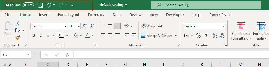
As its name implies, this toolbar gives quick access to useful commands in Excel. And this can be customized!
For example, you may want to add the freeze panes command into the Quick Access Toolbar. To do so, click File > Options > Quick Access Toolbar.
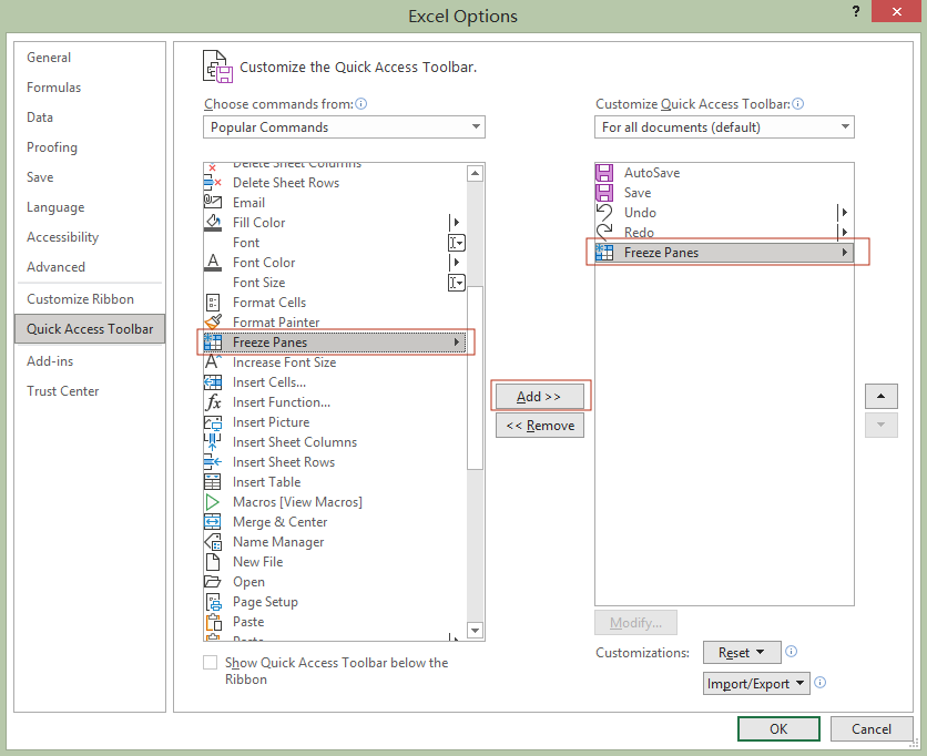
Here, select Freeze Panes in the list on the left side, then click on the Add button. This command will be added to the right-side list.
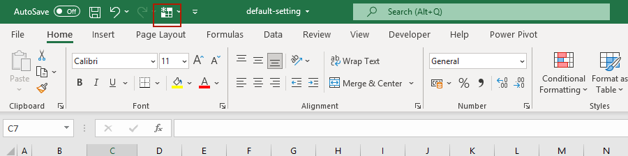
Press OK and the freeze panes command will appear in your Quick Access Toolbar!
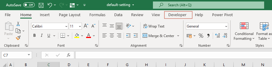
The Developer tab is hidden by default. Advanced users may want this displayed on the ribbon menu when working with macros. Here I will guide you to add this tab.
Click File > Options > Customize Ribbon, then check the "Developer" box in the "Main Tabs" list on the right side.
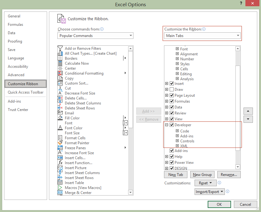
Press OK and the Developer tab will appear on the ribbon!
If you need to remove this tab, just uncheck the "Developer" box in the settings.
Macros are small computer programs that help you automate tasks within Excel. When you open a workbook containing macros, you may see a warning message:
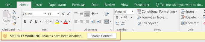
That's because Excel disable all macros by default. You can change this setting to enable macros all the time.
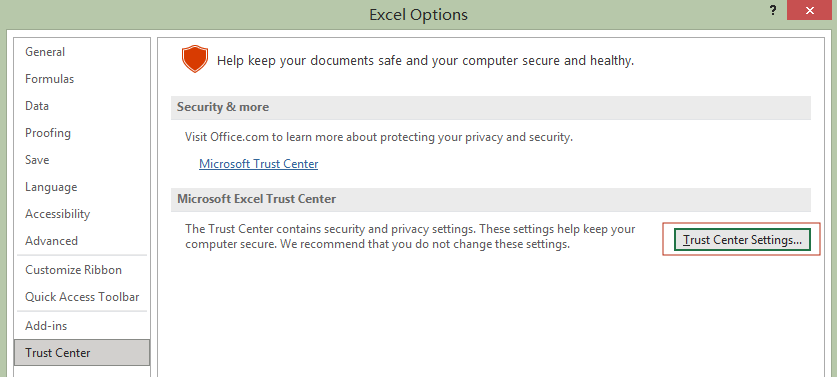
Click File > Options > Trust Center, then click on the Trust Center Settings button on the right side.
Once you are inside the Trust Center, click Macro Settings tab on the left. Here, select "Enable all macros" (not recommended; potentially dangerous code can run) option.
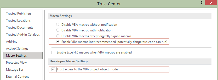
You may wonder if it's a good idea to activate this "not recommended" option. Great question, since macros can be dangerous if they are used to steal data or hijack computers.
If you only use macros occasionally, the second option "Disable all macros with notifications" may be more suitable.
But for heavy macro users, it makes sense to select "Enable all macros". Just keep in mind that with great power comes great responsibility, and be very careful about macros coming from other people.
And that's it for this tutorial! Now you can customize these settings and become an advanced user :-)
Here's a summary of the Excel settings covered in the second part of this tutorial:
Check out the other 5 useful settings in the first part of this tutorial if you haven't read it. If you know other great tips, feel free to let us know!