 ExcelFrog
Clear Excel Tutorials
ExcelFrog
Clear Excel Tutorials
When we want to extract specific values from a range in a Microsoft Excel file, the first thing that may come to mind is the VLOOKUP function. VLOOKUP is powerful but not very flexible. If you are tired of counting the number of rows or columns to put in your vlookups, this tutorial is for you!
We will learn how to perform advanced and dynamic lookups in Excel by combining two functions: INDEX and MATCH.
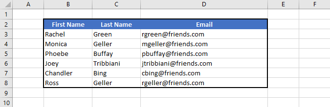
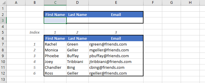
Here's the data that we'll work with. Our goal is to find a person's last name and email based on their first name.
Shall we begin?
Let's start with the INDEX function. It's used to retrieve a value at a given location in a range. The syntax looks like this:
=INDEX(lookup_range, row_number, column_number)
It has 3 parameters:
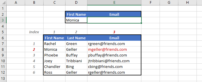
In our example, if we want to extract the email of Monica, we first need to set the lookup_range (C7:E12), then her email can be found in row_number (2) and column_number (3). So the formula would be:
=INDEX(C7:E12, 2, 3)
This works but it's not very dynamic. If we want to know Chandler's email, we have to change the row_number and column_number of the formula. That's pretty annoying! Fortunately we will be able to fix that with the MATCH function.
The MATCH function returns the relative position of a value in a given range. The syntax is:
=MATCH(lookup_value, lookup_range, match_type)
It also has 3 parameters:
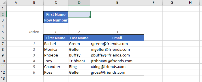
In our example, if we want to find the relative row number of the name Monica, we need to define the lookup_value (D2 a cell containing the string "Monica") and locate the lookup_range (C7:C12). We also set match_type to 0 to have an exact match.
=MATCH(D2, C7:C12, 0)
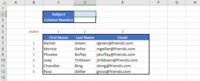
Note that the MATCH function is quite flexible. We can either do it in a vertical range to retrieve a row number (like we just did) or in a horizontal range to retrieve a column number. If we wanted to retrieve the column number of a given subject in the cell D2, the formula would be:
=MATCH(D2, C6:E6, 0)
In order to avoid unnecessary errors and mismatches, I highly recommend to set match_type all the time even though this parameter is optional.
Remember the problem mentioned in our INDEX example earlier? Our formula was not flexible since we needed to enter hard-coded values for the row and column numbers. Now with the help of the MATCH function, we can do something much more dynamic!
Here's the idea. We will put MATCH inside the INDEX function to find the row and column numbers of our lookup value dynamically. So the formula will be:
=INDEX(C7:E12, MATCH(C3, C7:C12, 0), MATCH(E2, C6:E6, 0))
That's a large formula! But don't worry, it will make sense with our example.
We want to get the email for a given first name. When we type "Monica" in the cell C3, the first MATCH will return 2 as the row number of Monica and the second MATCH will return 3 as the column number of the email. The big formula becomes:
=INDEX(C7:E12, 2, 3)
So we look at the 2nd row and 3rd column in the range C7:E12, which is the email of Monica!
Now if we are interested in the email of Joey, we just need to change cell C3 to "Joey", and boom, we get his email. The position of the lookup value is located dynamically in the lookup range, that's the magic of combining INDEX and MATCH.
Here's why INDEX MATCH is Better than VLOOKUP:
As an advanced Excel user, I believe using INDEX MATCH instead of VLOOKUP is one of the best practices to follow.
Here's a quick summary of what we've covered:
=INDEX(lookup_range, row_number, column_number)
=MATCH(lookup_value, lookup_range, match_type)
=INDEX(range, MATCH(lookup_value, lookup_range, type), MATCH(lookup_value, lookup_range, type))
Let's forget VLOOKUP, all you need is INDEX MATCH! This will be your secret weapon to impress any Excel user :-)