ExcelFrog Clear Excel Tutorials

home about

Excel: Make Your Data Visual With Conditional Formatting

Once you have important data in Microsoft Excel, it's time to analyze it. But it can be hard to understand the data when it's just plain numbers on top of each other. A good way to solve this is to make your data visual, and that's what we are going to cover in this short tutorial with conditional formatting.

Here's the data we are going to play with.

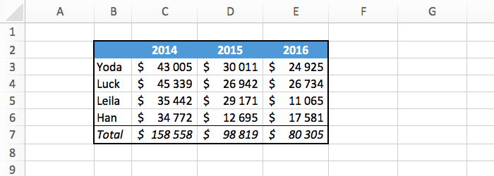
From this alone, it's hard to quickly see which years are bad, average, or good. Let's try to fix that!

Color Scales

Conditional formatting makes the formatting of the cells dynamic, based on their values. And it's super simple to use.

Select all the numbers, click on the "conditional formatting" button, select "color scales", and use the third one. You can try the other color schemes, but the third is the one that I recommend.

A cell in green has a high value, and a cell in red has a low value.

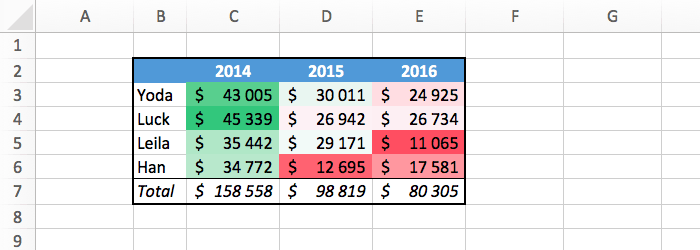
Now it's obvious to see which months are bad/average/good. And if you ever change your data, the formatting will be updated directly.

Greater Than

The downside of the above method is that it adds a lot of colors to your table, and that can make things a little messy. You can fix that if you are looking for something more specific, like knowing which cells are higher than 30,000.

This time do: "conditional formatting" > "highlight cell rules" > "greater than". In the popup that appears you need to enter the number you are looking for (30,000) and what formatting to apply (green).

And ta-da, you get to see exactly what you wanted, without cluttering the data too much.

Feel free to explore the other rules available in the menu. For example you could format the cells lower than 20,000 in red, or make the cells exactly equal to zero in yellow.

Clear Formatting

To remove a conditional formatting, follow these steps.

Select your data, then in the "conditional formatting" menu do "clear rules" > "clear rules from selected cells".

Conclusion

With these new ways to look at your data, you can quickly understand any table full of numbers.

Here's a quick summary of what we covered:

• Color scales: "conditional formatting" > "color scales" > click on the third one.
• Greater than: "conditional formatting" > "highlight cell rules" > "greater than".
• Remove formatting: "conditional formatting" > "clear rules" > "clear rules from selected cells".

See all the tutorials on the homepage